how to freeze row in excel
Select the third column. Here is how to do it.
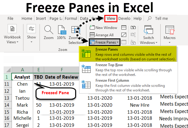
Freeze Panes In Excel How To Freeze Panes In Excel
When freezing a rows and columns at the same time click on the one cell located just below and to the right of the rows and columns you want frozen.
. How To Freeze Top Row And First Two Columns In Excel 2010. Skip to content Menu Menu Computing Gaming PC Guide Best Gaming PC Best 2000 Gaming PC Best 1000 Gaming PC Best 600 Gaming PC Best 300 Gaming PC Tablet PC Guide Best 10 Inch Tablet Best Tablet For Gaming. Select View Freeze Panes Freeze First Column.
For example to freeze top two rows in Excel we select cell A3 or the entire row 3 and click Freeze Panes. Excel How To Freeze Top Row And First Two Columns. First lets see how you can freeze a single row of data.
Freeze columns and rows. When the columns towards the right side are empty youll observe that the cell border of the Columns will be. Freeze The First Column.
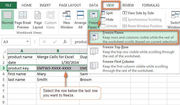
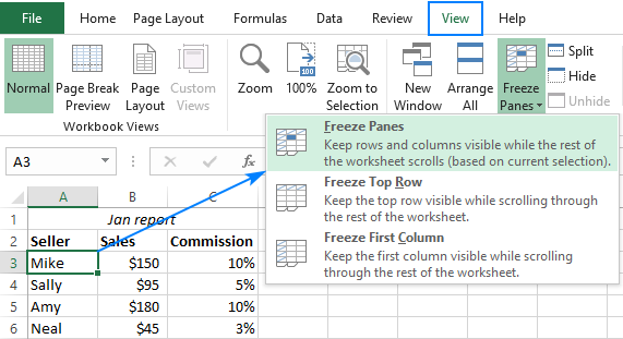
Next switch to the View tab click the Freeze Panes dropdown menu and then click Freeze Panes Now as you scroll down the sheet rows one through five are frozen. The faint line that appears between Column A and B shows that the first column is frozen. This is usually the top row in your workbook.
Excel 2013 and Excel 2010. Select the Freeze Panes option under it. When you lot work with a large Excel worksheet its often difficult to remember exactly what kind of data columns or rows incorporate once you begin scrolling around the sail.
Note that a thick gray line. How to Freeze a Single Row on Excel. How To Do This.
For example if you want to freeze the first 3 columns A C select the entire column D or cell D1. Click the small arrow next to the icon to see all the options. How to freeze a row in excel that isnt the top row.
Apart from that you can freeze the top row only regardless of where the position of the cursor is using a keyboard shortcut that is Alt-W-F-R. To select the row just click the number to the left of the row. How do I filter data in Excel with multiple criteria.
How To Freeze Panes In Excel Lock Rows And Columns. After selecting your row navigate to View in the header toolbar and select Freeze Panes. With the freeze panes option Excel freezes the rows and columns preceding the current active cell.
To freeze the acme row or first column. Freeze the first two columns. And now follow the already familiar path ie View tab Freeze panes and again Freeze panes.
Select the Row under the rows you would like to freeze by clicking on the row number to the left of each row. Open the sheet where in you want to freeze the multiple rows and columns keep the first row on top and first column to the left then click next to the cell of the last column and row till where you want to freeze as an example we would like to freeze from Row 1 to 13 and Column A to E so we will click on Cell F14. How to make header row sticky in excel.
Freeze rows or columns. Select the Freeze Top Row option or Freeze First Column depending on how you want to organize your data. Freeze the top row so you can see the header and know what youre looking at as you scroll.
This is helpful if you want to freeze a specific row for whatever reason. A grey line will appear to show what rows will be frozen in place. Open the View tab in Excel and look for the Freeze Panes command icon in the Window group.
For example if you want to freeze row 1 select row 2. Other than the first row you can freeze any single row you want. How To Freeze Top Row And First Column In Excel At Same Time.
To others its Serious Business. For the Address example we would click on Row 3 because we want to view Rows 1 and 2. Select the same number of rows above which you want to add new onesRight-click the selection and then select Insert Rows.
Freeze rows in Excel. For this example Im selecting row number three to freeze row number two. Under the VIEW tab select FREEZE PANES.
Select the column to the right of the last column you want to freeze. Go to the View tab. Learning how to freeze a row in Excel will work wonders for the readability of spreadsheets and workbooks.
Open the Excel workbook. Select the entire row below the row you want to freeze. Check How to Use the Average Function in Excel here.
Freeze the first column. To freeze a specific row in Excel select the row number immediately underneath the one you want frozen. Select FREEZE PANES again.
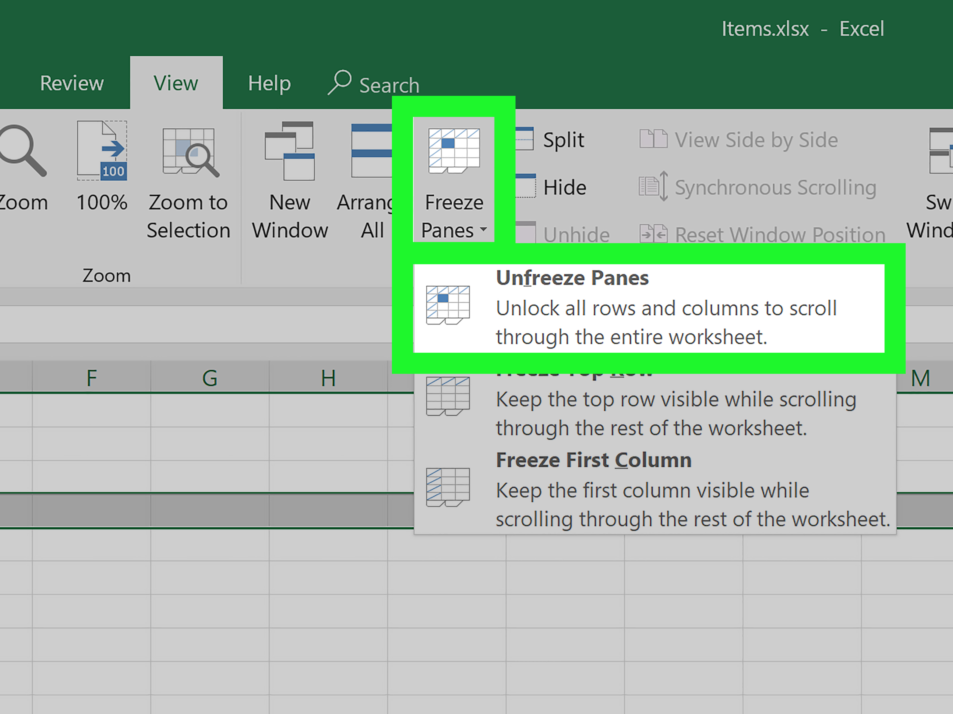
Or apply sticky notes for the cell that remain visible in the sheet with a line indicating the cell. Excel will automatically add a dark grey horizontal line that indicates that the top row is now frozen. Select View Freeze Panes Freeze Panes.
The cell_format parameter will be applied to any cells in the row that dont have a format. Click on the Freeze Panes option. With that the.
Each sheet has columns addressed by letters starting at A. Select the row or the first cell in the row right below the last row you want to freeze. How to freeze multiple columns in Excel.
On the View tab click Freeze Panes Freeze Panes. The shortcut to freeze the row and column together is AltWFF when pressed one by. Find out how here.
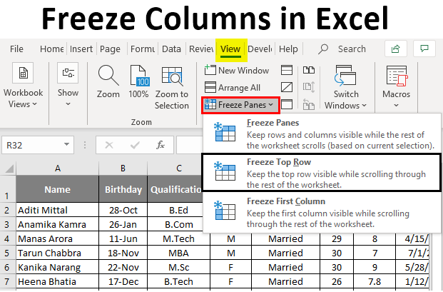
Freeze Columns In Excel Examples On How To Freeze Columns In Excel
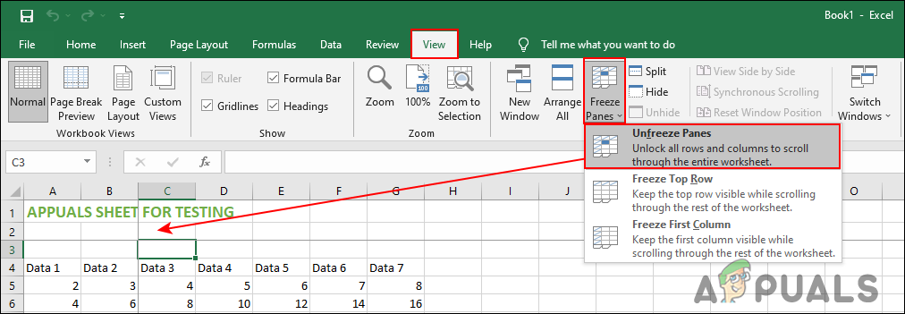
How To Freeze Row And Column In Microsoft Excel Appuals Com
How To Freeze Panes In Excel Lock Rows And Columns Ablebits Com
How To Freeze Cells In Excel

Freeze Panes To Lock Rows And Columns
How To Freeze A Row In Excel So It Always Stays Visible
How To Freeze Rows And Columns In Excel
How To Freeze A Row In Excel So It Always Stays Visible
0 Response to "how to freeze row in excel"
Post a Comment